In this post, I’ll walk through the mathematical formalism of reverse-mode automatic differentiation (AD) and try to explain some simple implementation strategies for reverse-mode AD. Demo programs in Python and Rust are included.
A simple example
Suppose we want to calculate the expression:
\[z = x \cdot y + \sin(x)\]
To do this using a program, we’d just translate it directly to code:
What if we’re also interested in the derivatives of \(z\)? The “obvious” approach is to just find the expression by hand (or using a computer algebra system) and then punch it into the computer as we did before. But that assumes we have an explicit form for \(z\). What if all we had was a program?
The important realization that leads to automatic differentiation is the fact that even biggest, most complicated program must be built from a small set of primitive operations such as addition, multiplication, or trigonometric functions. The chain rule allows us to take full advantage of this property.
Forward-mode automatic differentiation
First, we need to think about how a computer would evaluate \(z\) via a sequence of primitive operations (multiplication, sine, and addition):
The question marks indicate that x and y are to be supplied by the user.
I was careful to avoid reassigning to the same variable: this way we can treat each assignment as a plain old math equation:
\[\begin{align} x &= {?} \\ y &= {?} \\ a &= x \cdot y \tag{A} \\ b &= \sin(x) \\ z &= a + b \end{align}\]
Let’s try to differentiate each equation with respect to some yet-to-be-given variable \(t\):
\[\begin{align} \frac{\partial x}{\partial t} &= {?} \tag{F1} \\ \frac{\partial y}{\partial t} &= {?} \\ \frac{\partial a}{\partial t} &= y \cdot \frac{\partial x}{\partial t} + x \cdot \frac{\partial y}{\partial t} \\ \frac{\partial b}{\partial t} &= \cos(x) \cdot \frac{\partial x}{\partial t} \\ \frac{\partial z}{\partial t} &= \frac{\partial a}{\partial t} + \frac{\partial b}{\partial t} \end{align}\]
To obtain this, I have made liberal use of the chain rule:
\[\begin{align} \frac{\partial w}{\partial t} &= \sum_i \left(\frac{\partial w}{\partial u_i} \cdot \frac{\partial u_i}{\partial t}\right) \tag{C1} \\ &= \frac{\partial w}{\partial u_1} \cdot \frac{\partial u_1}{\partial t} + \frac{\partial w}{\partial u_2} \cdot \frac{\partial u_2}{\partial t} + \cdots \end{align}\]
where \(w\) denotes some output variable and \(u_i\) denotes each of the input variables that \(w\) depends on.
If we substitute \(t = x\) into equations (F1), we’d have an algorithm for calculating \(\partial z / \partial x\). Alternatively, to get \(\partial z / \partial y\), we could just plug in \(t = y\) instead.
Now, let’s translate the equations (F1) back into an ordinary program involving the differential variables {dx, dy, …}, which stand for \(\{\partial x / \partial t, \partial y / \partial t, \ldots\}\) respectively:
If we substitute \(t = x\) into the mathematical equations, what happens to this program? The effect is remarkably simple: we just need to initialize dx = 1 and dy = 0 as the seed values for the algorithm. Hence, by choosing the seeds dx = 1 and dy = 0, the variable dz will contain the value of the derivative \(\partial z / \partial x\) upon completion of the program. Similarly, if we want \(\partial z / \partial y\), we would use the seed dx = 0 and dy = 1 and the variable dz would contain the value of \(\partial z / \partial y\).
So far we have shown how the derivative can be calculated for a specific function like our example. To make the process fully automatic, we prescribe a set of rules for translating a program that evaluates an expression (like Program A) into a program that evaluates its derivatives (like Program B). We have already discovered 3 of these rules, in fact:
This can be extended further for subtraction, division, powers, other trigonometric functions, etc using multivariable calculus:
c = a - b     =>    dc = da - db
c = a / b     =>    dc = da / b - a * db / b ** 2
c = a ** b    =>    dc = b * a ** (b - 1) * da + log(a) * a ** b * db
c = cos(a)    =>    dc = -sin(a) * da
c = tan(a)    =>    dc = da / cos(a) ** 2
To translate using the rules, we simply replace each primitive operation in the original program by its differential analog. The order of the program remains unchanged: if a statement K is evaluated before another statement L, then the differential analog of statement K is still evaluated before the differential analog of statement L. This is forward-mode automatic differentiation.
A careful inspection of Program A and Program B reveals that it is actually possible to interleave the differential calculations with the original calculations:
x  = ?
dx = ?

y  = ?
dy = ?

a  = x * y
da = y * dx + x * dy

b  = sin(x)
db = cos(x) * dx

z  = a + b
dz = da + db
This demonstrates the two main advantages of forward-mode AD:
- The differential variables usually depend on the intermediate variables, so if we do them together there’s no need to hold on to the the intermediate variables until later, saving memory.
- This enables an implementation using dual numbers. In languages with operator overloading, this translates to a very simple, direct implementation of forward-mode AD.
For an example in Rust, see the rust-ad library.
Reverse-mode automatic differentiation
The implementation simplicity of forward-mode AD comes with a big disadvantage, which becomes evident when we want to calculate both \(\partial z/\partial x\) and \(\partial z/\partial y\). In forward-mode AD, doing so requires seeding with dx = 1 and dy = 0, running the program, then seeding with dx = 0 and dy = 1 and running the program again. In effect, the cost of the method scales linearly as O(n) where n is the number of input variables. This would be very costly if we wanted to calculate the gradient of a large complicated function of many variables, which happens surprisingly often in practice.
Let’s take a second look at the chain rule (C1) we used to derive forward-mode AD:
\[\begin{align} \frac{\partial w}{\partial t} &= \sum_i \left(\frac{\partial w}{\partial u_i} \cdot \frac{\partial u_i}{\partial t}\right) \tag{C1} \\ &= \frac{\partial w}{\partial u_1} \cdot \frac{\partial u_1}{\partial t} + \frac{\partial w}{\partial u_2} \cdot \frac{\partial u_2}{\partial t} + \cdots \end{align}\]
To calculate the gradient using forward-mode AD, we had to perform two substitutions: one with \(t = x\) and another with \(t = y\). This meant we had to run the entire program twice.
However, the chain rule is symmetric: it doesn’t care what’s in the “numerator” or the “denominator”. So let’s rewrite the chain rule but turn the derivatives upside down:
\[\begin{align} \frac{\partial s}{\partial u} &= \sum_i \left(\frac{\partial w_i}{\partial u} \cdot \frac{\partial s}{\partial w_i}\right) \tag{C2} \\ &= \frac{\partial w_1}{\partial u} \cdot \frac{\partial s}{\partial w_1} + \frac{\partial w_2}{\partial u} \cdot \frac{\partial s}{\partial w_2} + \cdots \end{align}\]
In doing so, we have inverted the input-output roles of the variables. The same naming convention is used here: \(u\) for some input variable and \(w_i\) for each of the output variables that depend on \(u\). The yet-to-given variable is now called \(s\) to highlight the change in position.
In this form, the chain rule could be applied repeatedly to every input variable \(u\), akin to how in forward-mode AD we applied the chain rule repeatedly to every output variable \(w\) to get equation (F1). Therefore, given some \(t\), we expect a program that uses chain rule (C2) to be able to compute both \(\partial s / \partial x\) and \(\partial s / \partial y\) in one go!
So far, this is just a hunch. Let’s try it on the example problem (A).
\[\begin{align} \frac{\partial s}{\partial z} &= {?} \tag{R1} \\ \frac{\partial s}{\partial b} &= \frac{\partial s}{\partial z} \\ \frac{\partial s}{\partial a} &= \frac{\partial s}{\partial z} \\ \frac{\partial s}{\partial y} &= x \cdot \frac{\partial s}{\partial a} \\ \frac{\partial s}{\partial x} &= y \cdot \frac{\partial s}{\partial a} + \cos(x) \cdot \frac{\partial s}{\partial b} \end{align}\]
If you haven’t done this before, I suggest taking the time to actually derive these equations using (C2). It can be quite mind-bending because everything seems “backwards”: instead of asking what input variables a given output variable depends on, we have to ask what output variables a given input variable can affect. The easiest way to see this visually is by drawing a dependency graph of the expression:
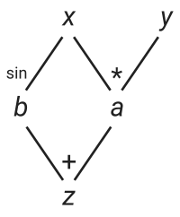
The graph shows that
- the variable
adirectly depends onxandy, - the variable
bdirectly depends onx, and - the variable
zdirectly depends onaandb.
Or, equivalently:
- the variable
bcan directly affectz, - the variable
acan directly affectz, - the variable
ycan directly affecta, and - the variable
xcan directly affectaandb.
Let’s now translate the equations (R1) into code. As before, we replace the derivatives \(\{\partial s / \partial z, \partial s / \partial b, \ldots\}\) by variables {gz, gb, …}, which we call the adjoint variables. This results in:
Going back to the equations (R1), we see that if we substitute \(s = z\), we would obtain the gradient in the last two equations. In the program, this is equivalent to setting gz = 1 since gz is just \(\partial s / \partial z\). We no longer need to run the program twice! This is reverse-mode automatic differentiation.
There is a trade-off, of course. If we want to calculate the derivative of a different output variable, then we would have to re-run the program again with different seeds, so the cost of reverse-mode AD is O(m) where m is the number of output variables. If we had a different example such as:
\[\begin{cases} z = 2 x + \sin(x) \\ v = 4 x + \cos(x) \end{cases}\]
in reverse-mode AD we would have to run the program with gz = 1 and gv = 0 (i.e. \(s = z\)) to get \(\partial z / \partial x\), and then rerun the program with gz = 0 and gv = 1 (i.e. \(s = v\)) to get \(\partial v / \partial x\). In contrast, in forward-mode AD, we’d just set dx = 1 and get both \(\partial z / \partial x\) and \(\partial v / \partial x\) in one run.
There is a more subtle problem with reverse-mode AD, however: we can’t just interleave the derivative calculations with the evaluations of the original expression anymore, since all the derivative calculations appear to be going in reverse to the original program. Moreover, it’s not obvious how one would even arrive at this point in using a simple rule-based algorithm – is operator overloading even a valid strategy here? How do we put the “automatic” back into reverse-mode AD?
A simple implementation in Python
One way is to parse the original program and then generate an adjoint program that calculates the derivatives. This is usually quite complicated to implement, and its difficulty varies significantly depending on the complexity of the host language. Nonetheless, this may be worthwhile if efficient is critical, as there are more opportunities to perform optimizations in this static approach.
A simpler way is to do this dynamically: construct a full graph that represents our original expression as as the program runs. The goal is to get something akin to the dependency graph we drew earlier:
The “roots” of the graph are the independent variables x and y, which could also be thought of as nullary operations. Constructing these nodes is a simple matter of creating an object on the heap:
class Var:
    def __init__(self, value):
        self.value = value
        self.children = []
        …
    …

# define the Vars for the example problem
# initialize x = 0.5 and y = 4.2
x = Var(0.5)
y = Var(4.2)
What does each Var node store? Each node can have several children, which are the other nodes that directly depend on that node. In the example, x has both a and b as its children. Cycles are not allowed in this graph.
By default, a node is created without any children. However, whenever a new expression \(u\) is built out of existing nodes \(w_i\), the new expression \(u\) registers itself as a child of each of its dependencies \(w_i\). During the child registration, it will also save its contributing weight
\[\frac{\partial w_i}{\partial u}\]
which will be used later to compute the gradients. As an example, here is how we would do this for multiplication:
class Var:
    …
    def __mul__(self, other):
        z = Var(self.value * other.value)
        self.children.append((other.value, z)) # weight = ∂z/∂self = other.value
        other.children.append((self.value, z)) # weight = ∂z/∂other = self.value
        return z
    …

…
# “a” is a new Var that is a child of both x and y
a = x * y
As you can see, this method, like most dynamic approaches for reverse-mode AD, requires doing a bunch of mutation under the hood.
Finally, to get the derivatives, we need to propagate the derivatives. This can be done using recursion, starting at the roots x and y. To avoid unnecessarily traversing the tree multiple times, we cache the value of in an attribute called grad_value.
class Var:
    def __init__(self):
        …
        # initialize to None, which means it’s not yet evaluated
        self.grad_value = None

    def grad(self):
        # recurse only if the value is not yet cached
        if self.grad_value is None:
            # calculate derivative using chain rule
            self.grad_value = sum(weight * var.grad()
                                  for weight, var in self.children)
        return self.grad_value
    …

…
a.grad_value = 1.0
print("∂a/∂x = {}".format(x.grad())) # ∂a/∂x = 4.2
Here is the complete demonstration of this approach in Python.
Note that because we are mutating the grad_value attribute of the nodes, we can’t reuse the tree to calculate the derivative of a different output variable without traversing the entire tree and resetting every grad_value attribute to None.
A tape-based implementation in Rust
The approach described is not very efficient: a complicated expression can contain lots of primitive operations, leading to lots of nodes being allocated on the heap.
A more space-efficient way to do this is to create nodes by appending them to an existing, growable array. Then, we could just refer to each node by its index in this growable array. Note that we do not use pointers here! If the vector’s capacity changes, pointers to its elements would become invalid.
Using a vector to store nodes does a great job at reducing the number of allocations, but, like any arena allocation method, we won’t be able to deallocate portions of the graph. It’s all or nothing.
Also, we need to somehow fit each node into a fixed amount of space. But then how would we store its list of children?
Turns out, we don’t actually need to store the children. Instead, each node could just store indices to their parent nodes. Conceptually, it would look like this for our example problem:
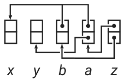
Note the similarity with the graph earlier.
In Rust, we can describe each node using a structure containing two weights and two parent indices:
You might wonder why we picked two. This is because we are assuming all primitive operations are binary. For example, the node for the variable a = x * y would look like:
But there’s unary and nullary operations too − how will we deal with those? Quite easy actually, we just set the weights to zero. For example, the node for the variable b = sin(x) would look like:
As a convention, we will put the index of the node itself into /* whatever */. It really doesn’t matter what we put in there as long as the index is not out of bounds.
The nodes themselves are stored in a common array (Vec<Node>) that is shared by the entire expression graph, which also acts as the allocation arena. In AD literature, this shared array is often called a tape (or Wengert list). The tape can be thought of as a record of all the operations performed during the evaluation of the expression, which in turn contains all the information required to compute its gradient when read in reverse.
In the Python implementation, the nodes were identified with expressions: nodes can be directly combined via arithmetic operations to form new nodes. In Rust, we treat the nodes and expressions as separate entities. Nodes exist solely on the tape, while expressions are just thin wrappers over node indices. Here is what the expression type looks like:
The expression type contains a pointer to the tape, an index to the node, and an associated value. Note that the expression satisfies Copy, which allows it to be duplicated freely without regard. This is necessary to maintain the illusion that the expression acts like an ordinary floating-point number.
Also, note that the tape is an immutable pointer. We need to modify the tape as we build the expression, but we are going to have lots of expressions holding a pointer to the same tape. This won’t work with a mutable pointer, since they are exclusive, so we must “cheat” Rust’s read-write-lock system using a RefCell:
The bulk of the implementation work lies in coding up the primitive operations. Here’s what the unary sin function looks like:
impl<'t> Var<'t> {
    pub fn sin(self) -> Self {
        Var {
            tape: self.tape,
            value: self.value.sin(),
            index: self.tape.push1(
                self.index, self.value.cos(),
            ),
        }
    }
}
Any unary function can be implemented just like this. Here, push1 is a helper function that constructs the node, pushes it onto the tape, and then returns the index of this new node:
impl Tape {
    fn push1(&self, dep0: usize, weight0: f64) -> usize {
        let mut nodes = self.nodes.borrow_mut();
        let len = nodes.len();
        nodes.push(Node {
            weights: [weight0, 0.0],
            deps: [dep0, len],
        });
        len
    }
}
Finally, when it’s time to do the derivative calculation, we need to traverse the entire tape in reverse and accumulate the derivatives using the chain rule. This is done by the grad function associated with the Var object:
impl<'t> Var<'t> {
    pub fn grad(&self) -> Grad {
        let len = self.tape.len();
        let nodes = self.tape.nodes.borrow();

        // allocate the array of derivatives (specifically: adjoints)
        let mut derivs = vec![0.0; len];

        // seed
        derivs[self.index] = 1.0;

        // traverse the tape in reverse
        for i in (0 .. len).rev() {
            let node = nodes[i];
            let deriv = derivs[i];

            // update the adjoints for its parent nodes
            for j in 0 .. 2 {
                derivs[node.deps[j]] += node.weights[j] * deriv;
            }
        }

        Grad { derivs: derivs }
    }
}
The crucial part lies in the loop. Here, we do not sum over all the derivatives at the same time like in chain rule (C2) or like in the Python program. Rather, we break chain rule up into a sequence of addition-assignments:
\[\frac{\partial s}{\partial u} \leftarrow \frac{\partial s}{\partial u} + \frac{\partial w_i}{\partial u} \frac{\partial s}{\partial w_i}\]
The reason we’re doing this is because we don’t keep track of children anymore. So rather than accumulating all the derivatives contributed by each child all at once, we let each node make its contributions to their parents at their own pace.
Another major difference from the Python program is that the derivatives are now stored on a separate array derivs, which is then disguised as a Grad object:
This means that, unlike the Python program, where all the derivatives are stored in the grad_value attribute of each node, we have decoupled the tape from the storage of the derivatives, allowing the tape / expression graph to be re-used for multiple reverse-mode AD calculations (in case we have multiple output variables).
The derivs array contains all the adjoints / derivatives at the same index as its associated node. Hence, to get the adjoint of a variable whose node is located at index 3, we just need to grab the element the derivs array at index 3. This is implemented by the wrt (“with respect to”) function of the Grad object:
Here’s the full demonstration of reverse-mode AD in Rust. To use this rudimentary AD library, you would write:
let t = Tape::new();

let x = t.var(0.5);
let y = t.var(4.2);

let z = x * y + x.sin();

let grad = z.grad();

println!("z = {}", z.value);         // z = 2.579425538604203
println!("∂z/∂x = {}", grad.wrt(x)); // ∂z/∂x = 5.077582561890373
println!("∂z/∂y = {}", grad.wrt(y)); // ∂z/∂y = 0.5
Total differentials and differential operators
Notice that if we throw away the \(\partial t\) from the denominators of equation (F1), we end up with a set of equations relating the total differentials of each variable:
\[\begin{align} \mathrm{d} x &= {?} \\ \mathrm{d} y &= {?} \\ \mathrm{d} a &= y \cdot \mathrm{d} x + x \cdot \mathrm{d} y \\ \mathrm{d} b &= \cos(x) \cdot \mathrm{d} x \\ \mathrm{d} z &= \mathrm{d} a + \mathrm{d} b \end{align}\]
This is why variables such as dx are called “differentials”. We can also write chain rule (C1) in a similar form:
\[\mathrm{d} w = \sum_i \left(\frac{\partial w}{\partial u_i} \cdot \mathrm{d} u_i\right)\]
Similarly, we can throw away the \(s\) in equation (R1), which then becomes an equation of differential operators:
\[\begin{align} \frac{\partial}{\partial z} &= {?} \\ \frac{\partial}{\partial b} &= \frac{\partial}{\partial z} \\ \frac{\partial}{\partial a} &= \frac{\partial}{\partial z} \\ \frac{\partial}{\partial y} &= x \cdot \frac{\partial}{\partial a} \\ \frac{\partial}{\partial x} &= y \cdot \frac{\partial}{\partial a} + \cos(x) \cdot \frac{\partial}{\partial b} \end{align}\]
We can do the same for (C2):
\[\frac{\partial}{\partial u} = \sum_i \left(\frac{\partial w_i}{\partial u} \cdot \frac{\partial}{\partial w_i}\right) \tag{C4}\]
Saving memory via a CTZ-based strategy
OK, this section is not really part of the tutorial, but more of a discussion regarding a particular optimization strategy that I felt was interesting enough to deserve some elaboration (it was briefly explained on in a paper by Griewank).
So far, we have resigned ourselves to the fact that reverse-mode AD requires storage proportional to the number of intermediate variables.
However, this is not entirely true. If we’re willing to repeat some intermediate calculations, we can make do with quite a bit less storage.
Suppose we have an expression graph that is more or less a straight line from input to output, with N intermediate variables lying in between. So this is not so much an expression graph anymore, but a chain. In the naive solution, we would require O(N) storage space for this very long expression chain.
Now, instead of caching all the intermediate variables, we construct a hierarchy of caches and maintain this hierachy throughout the reverse sweep:
cache_0stores the initial valuecache_1stores the result halfway down the chaincache_2stores the result 3/4 of the way down the chaincache_3stores the result 7/8 of the way down the chaincache_4stores the result 15/16 of the way down the chain- …
Notice that the storage requirement is reduced to O(log(N)) because we never have more than log2(N) + 1 values cached.
During the forward sweep, maintaining such a hierarchy would require evicting older cache entries at an index determined by a formula that involves the count-trailing-zeros function.
The easiest way to understand the CTZ-based strategy is to look at an example. Let’s say we have a chain of 16 operations, where 0 is the initial input and f is the final output:
0 1 2 3 4 5 6 7 8 9 a b c d e fSuppose we have already finished the forward sweep from 0 to f. In doing so, we have cached 0, 8, c, e, and f:
 0 1 2 3 4 5 6 7 8 9 a b c d e f
                                ^
 X---------------X-------X---X-X
The X symbol indicates that the result is cached, while ^ indicates the status of our reverse sweep. Now let’s start moving backward. Both e and f are available so we can move past e without issue:
 0 1 2 3 4 5 6 7 8 9 a b c d e f
                            ^
 X---------------X-------X---X-X
Now we hit the first problem: we are missing d. So we recompute d from c:
 0 1 2 3 4 5 6 7 8 9 a b c d e f
                            ^
 X---------------X-------X---X-X
                         |
                         +-X
We then march on past c.
 0 1 2 3 4 5 6 7 8 9 a b c d e f
                        ^
 X---------------X-------X---X-X
                         |
                         +-X
Now we’re missing b. So we recompute starting at 8, but in doing so we also cache a:
 0 1 2 3 4 5 6 7 8 9 a b c d e f
                        ^
 X---------------X-------X---X-X
                 |       |
                 +---X-X +-X
We continue on past a:
 0 1 2 3 4 5 6 7 8 9 a b c d e f
                    ^
 X---------------X-------X---X-X
                 |       |
                 +---X-X +-X
Now 9 is missing, so recompute it from 8:
 0 1 2 3 4 5 6 7 8 9 a b c d e f
                    ^
 X---------------X-------X---X-X
                 |       |
                 +---X-X +-X
                 |
                 +-X
Then we move past 8:
 0 1 2 3 4 5 6 7 8 9 a b c d e f
                ^
 X---------------X-------X---X-X
                 |       |
                 +---X-X +-X
                 |
                 +-X
To get 7, we recompute starting from 0, but in doing so we also keep 4 and 6:
 0 1 2 3 4 5 6 7 8 9 a b c d e f
                ^
 X---------------X-------X---X-X
 |               |       |
 +-------X---X-X +---X-X +-X
                 |
                 +-X
By now you can probably see the pattern. Here are the next couple steps:
 0 1 2 3 4 5 6 7 8 9 a b c d e f
            ^
 X---------------X-------X---X-X
 |               |       |
 +-------X---X-X +---X-X +-X
         |       |
         +-X     +-X

 0 1 2 3 4 5 6 7 8 9 a b c d e f
        ^
 X---------------X-------X---X-X
 |               |       |
 +-------X---X-X +---X-X +-X
         |       |
         +-X     +-X

 0 1 2 3 4 5 6 7 8 9 a b c d e f
        ^
 X---------------X-------X---X-X
 |               |       |
 +-------X---X-X +---X-X +-X
 |       |       |
 +---X-X +-X     +-X

 0 1 2 3 4 5 6 7 8 9 a b c d e f
    ^
 X---------------X-------X---X-X
 |               |       |
 +-------X---X-X +---X-X +-X
 |       |       |
 +---X-X +-X     +-X

 0 1 2 3 4 5 6 7 8 9 a b c d e f
    ^
 X---------------X-------X---X-X
 |               |       |
 +-------X---X-X +---X-X +-X
 |       |       |
 +---X-X +-X     +-X
 |
 +-X

 0 1 2 3 4 5 6 7 8 9 a b c d e f
^
 X---------------X-------X---X-X
 |               |       |
 +-------X---X-X +---X-X +-X
 |       |       |
 +---X-X +-X     +-X
 |
 +-X
From here it’s fairly evident that the number of times the calculations get repeated is bounded by O(log(N)), since the diagrams above are just flattened binary trees and their height is bounded logarithmically.
Here is a demonstration of the CTZ-based chaining strategy.
As Griewank noted, this strategy is not the most optimal one, but it does have the advantage of being quite simple to implement, especially when the number of calculation steps is not known a priori. There are other strategies that you might find interesting in his paper.
For a more advanced review of automatic differentiation, see Bartholomew-Biggs et al “Automatic differentiation of algorithms”
Show Disqus comments
comments powered by Disqus